LLM ALIGNMENT

Alignment Data Map: Timing of SimPO Boundary Crossings and Model-Specific Differences

Ilho Ahn

Sep 01, 2026

Models trained on ADM HighAvg or Random data are compared on the same held-out preference pairs, tracing SimPO boundary crossings across model variants and checkpoints.

Lee et al.’s Alignment Data Map (ADM) [1] separates training data using the mean and variance of alignment scores computed over the candidate responses to an instruction. Its premise is that preference data do not all have equal learning value: mean response quality and variance across responses define the regions used for selection. The original study reported that training on only the 33% of samples in the high-mean, low-variance HighAvg region achieved alignment performance comparable to or better than training on the full dataset.

The selected training data and the pairs used to measure learning have different roles. This follow-up trains Qwen2.5-Instruct 1.5B, 3B, and 7B on either HighAvg or Random data, then tracks the same 600 held-out evaluation pairs under both policies. It asks whether the training-data choice changes when a policy first ranks an evaluation pair correctly or reaches the SimPO target margin.

Summary

• Separate instances of Qwen2.5-Instruct 1.5B, 3B, and 7B were trained under HighAvg and Random, using three seeds and 276 optimizer updates per condition. The trajectories belong to the same 600 held-out evaluation pairs, with no overlap with training.
• At all three model sizes, a larger proportion of pairs ended in an R/U/T state above their pre-training state under HighAvg than under Random. The advantage did not grow consistently with model size: it was largest for 7B, while the final difference for 3B was smaller than for 1.5B.
• The difference did not reflect small improvements across all pairs. Compared with Random, HighAvg had more movements across a boundary into a higher state, fewer positive margin changes confined to the same state, and some additional regressions.
• The clearest difference was that boundary-crossing upward passages were observed at earlier checkpoints under HighAvg within the same training budget. Random caught up on some pairs later in training, narrowing the final gap.
• These are changes in how policies score supplied responses. Crossing an objective boundary does not establish better generated answers or downstream tool use, which this comparison did not evaluate.

Problem Setting

ADM describes the measured properties of response sets and selects instructions for training. The unit of preference optimization is a prompt paired with chosen and rejected responses, constructed only after instruction selection. There is no reason to assume that the reference scorer used to select instructions and the model being trained find the same response pair equally difficult.

This distinction motivates the research question:

When training data come from HighAvg rather than Random, how do boundary crossings on a shared held-out evaluation set vary with the policy’s starting state, model variant, and training checkpoint?

The hypothesis examined here was that the effect of HighAvg might increase monotonically with model scale. If the selected training pairs contained subtle but useful distinctions, a larger model might learn from them more effectively.

Related Work

Differences Among Selection Criteria

The value of a preference pair can first be characterized by properties measured from the data itself. ADM separates instructions by the mean and variance of alignment scores over candidate responses [1]. Xiao et al. compared the positions of chosen and rejected responses within an on-policy reward distribution [2], while Deng et al. selected training data by combining an external reward margin with an implicit DPO margin [3].

Another axis is the learning state measured under the current policy. Yang et al. prioritized annotation for pairs with small implicit DPO reward margins under the policy and reference policy [4]. Huang et al. defined alignment potential as the gap between the current policy’s implicit margin and a target explicit margin [5]. A score gap is therefore not a universal measure of pair difficulty. Reference separation, policy-relative margin, and distance to a target provide different signals.

Time-Varying Value

The value of the same pair can also change during training. Peng et al.’s Uni-DPO adjusts weights using both intrinsic pair quality and the model’s evolving performance [6]. Li et al.’s MetaPO learns time-dependent sample weights from reward-margin evolution, learning volatility, and reference deviation [7]. A separate analysis connected input complexity and output ambiguity to different learning dynamics [8]. These studies share the view that a useful pair may depend on the current policy and the point in training.

Scope of This Analysis

This note compares models trained under fixed ADM selection conditions on an evaluation set separated from training. It tracks state transitions of those common evaluation pairs and the first observed upward passage within a limited update budget. The analysis evaluates the effect of training-data selection through held-out scoring trajectories; it does not propose a new selection rule or weighting method.

Experimental Setup

Data Selection and Training Comparison

In this note, HighAvg refers to preference pairs constructed from instructions selected from the high-mean, low-variance region of an ADM built with a fixed set of reference answers and a fixed scorer. Random refers to preference pairs constructed from instructions sampled at random from the same source pool.

The two conditions were constructed from the same source pool while preserving source and task composition, and were trained with the same LoRA and SimPO recipe. The training models were the official Qwen2.5-Instruct 1.5B, 3B, and 7B checkpoints. Three runs with different random seeds were conducted at each size. Both conditions used 276 optimizer updates and the same nominal batch budget, equivalent to approximately 3 epochs; this does not match the number of processed tokens or wall-clock compute.

A shared evaluation set of 600 pairs with no prompt or pair overlap with the training data was evaluated repeatedly at the base policy and at checkpoints at steps 92, 184, and 276. Keeping the same pairs made it possible to track not only endpoint aggregates but also the state into which each pair moved during training. This was a fixed development evaluation set used for the follow-up analysis, not a new blind test.

SimPO Margin and State Trajectory

This note uses training model to refer to the Qwen2.5-Instruct variant being trained (1.5B, 3B, or 7B), and policy to refer to $\pi_t$, which assigns response probabilities at a particular checkpoint.

For a pair $z=(x,y_w,y_l)$, the policy’s length-normalized log-probability margin is defined as

\[\Delta_{\pi}(z) = \frac{\log \pi(y_w\mid x)}{|y_w|} - \frac{\log \pi(y_l\mid x)}{|y_l|}.\]

Meng et al.’s SimPO [9] trains $\beta\Delta_{\pi}$ to exceed the target margin $\gamma$. With $\beta=2$ and $\gamma=1$ in this setup, the target boundary is $\Delta=0.5$. Each pair was therefore assigned to one of three states:

\[R:\Delta\le 0, \qquad U:0<\Delta<0.5, \qquad T:\Delta\ge0.5.\]

• R — reversed or tied: the rejected response ranks at least as high as the chosen response; ties at $\Delta=0$ are included.
• U — correct, below target: the chosen response ranks higher, but its separation is below the SimPO target.
• T — target satisfied: the chosen–rejected separation has reached the target.

Figure 1 shows how two objective boundaries divide the three states. Rightward movements R→U, R→T, and U→T were counted as upward transitions.

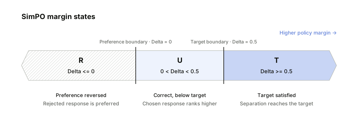
Figure 1. The R/U/T state space defined by the sign of the policy margin and the SimPO target boundary. Moving right increases the policy margin; arrows at the ends indicate that R and T are open-ended intervals. Segment widths do not encode numeric ranges or pair proportions.

Under this state definition, a pair for which the policy strongly prefers the rejected response may not cross the next boundary within a limited number of updates. A pair for which the policy already prefers the chosen response beyond the target margin has no higher R/U/T state to reach. Between them, the next preference or target-margin boundary may lie within reach, allowing the same pair to produce an upward state transition.

The first observed upward passage is the first evaluation checkpoint at which a state higher than the pre-training state is observed. State-standardized upward movement is the HighAvg-minus-Random difference in the proportion of pairs whose state at a given checkpoint is higher than at base, averaged over base-state-specific differences under a shared R/U/T distribution.

The model-size comparison reports observations from three official Qwen2.5-Instruct variants: 1.5B, 3B, and 7B. These model variants differ in training conditions and post-training outcomes as well as parameter count; this is not a controlled experiment in which only parameter count changes.

Results

Effects by Model Size and Training Checkpoint

At step 276, HighAvg showed higher reward accuracy, policy margin, final upward movement, and target reach than Random for all three seeds at all three model sizes, and lower SimPO loss. Appendix Table 2 records endpoint accuracy and loss differences by model and seed. These three training runs are shown individually rather than summarized as a seed-population confidence interval.

The effect size, however, did not follow the hypothesized monotonic order. After standardizing to a shared initial-state composition, the final HighAvg-minus-Random upward-movement differences were +5.64 pp for 1.5B, +4.27 pp for 3B, and +8.06 pp for 7B.

The checkpoint trajectories in Figure 2 show that the smaller effect for 3B than 1.5B at step 276 did not hold throughout training. For both 3B and 7B, the mean HighAvg-minus-Random difference peaked at step 184 and then declined at the final checkpoint. Across the three 3B seeds, the difference likewise grew during steps 92→184 and shrank during steps 184→276.

Figure 2. State-standardized HighAvg-minus-Random upward movement by model size and evaluation checkpoint. Gray circles denote 1.5B, blue squares 3B, and black diamonds 7B. Thin lines show individual seed trajectories and thick lines show their means. The mean final difference was smallest for 3B and largest for 7B; the mean differences for 3B and 7B both peaked at step 184.

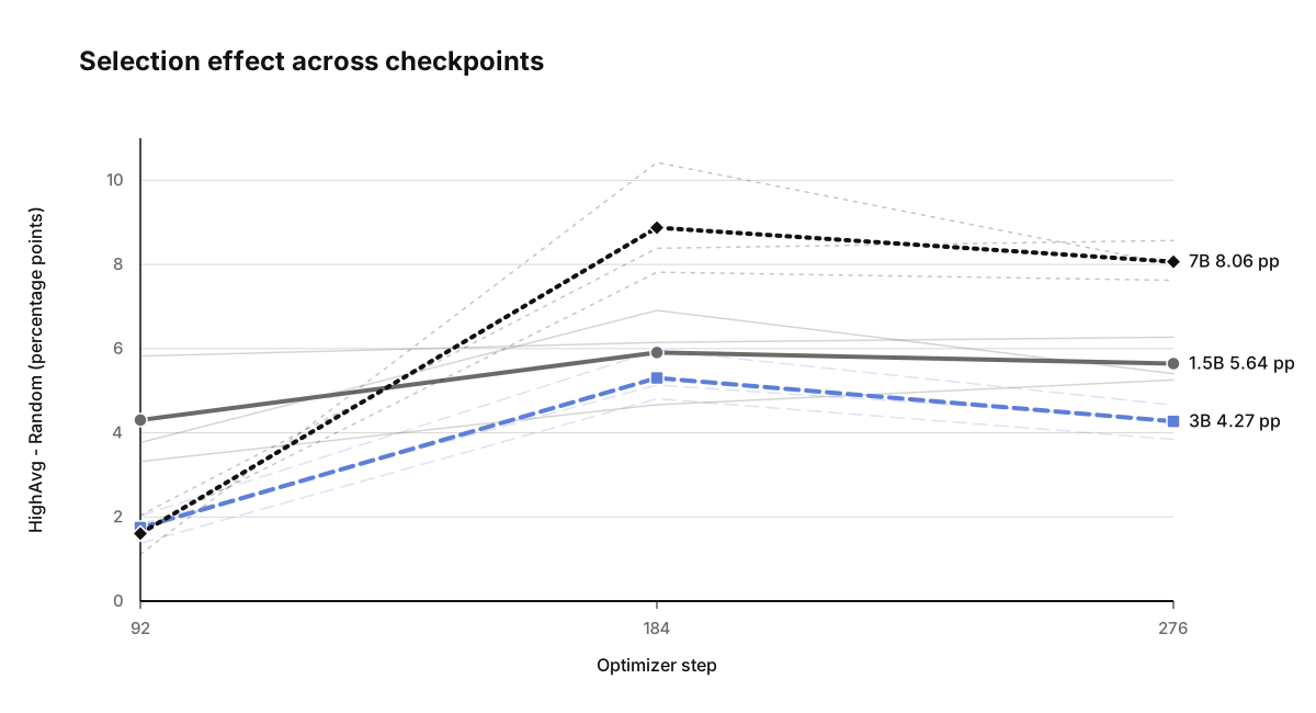
The HighAvg effect did not increase consistently with model size, and it varied with evaluation checkpoint within the same model. The initial R/U/T state of each pair and its distance to the next boundary therefore need to be considered alongside model size.

Endpoint Accuracy and Transition Composition

Reward accuracy counts only whether $\Delta>0$. It changes when a pair crosses the zero boundary, but it cannot reveal U→T, T→U, or margin changes within a state. It also does not preserve the path a pair took before the endpoint. The state decomposition therefore adds information that accuracy leaves out.

A detailed decomposition of same-pair training trajectories showed that HighAvg did not simply produce slightly larger margin gains across all pairs. At all three model sizes, fewer pairs stayed in the same state throughout training, while more pairs ended in a higher state without any downward transition or reached the target state by step 276. The changes were generally larger for 1.5B and 7B and smaller for 3B.

Not every movement was upward, as Figure 3 shows. At all three model sizes, the proportion of pairs that experienced at least one downward transition during training was also approximately 2 pp higher under HighAvg than Random. HighAvg was associated with state changes in more pairs, including some regressions.

At the pair level on the shared evaluation set, the difference between HighAvg and Random was clearer for movements that crossed a boundary into a higher state than for small margin increases within the same state. At every model size, more pairs showed this outcome only under HighAvg than only under Random. Pairs whose $\Delta$ increased without a state change were instead less common under HighAvg.

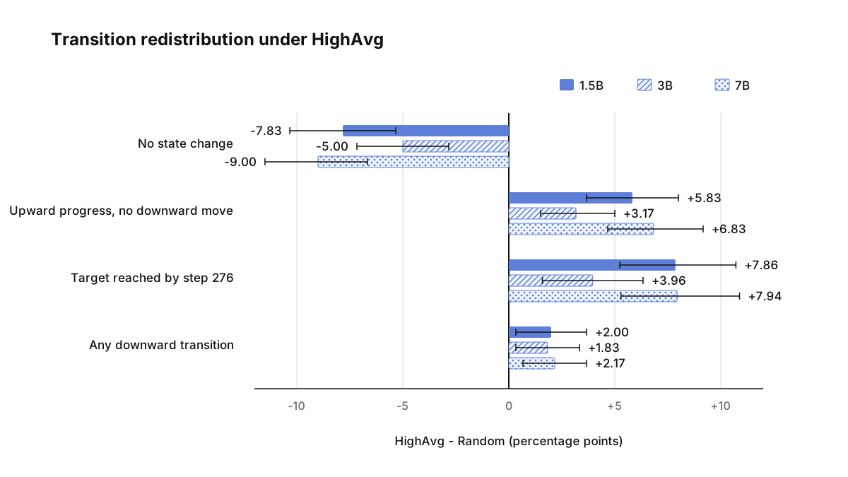
Figure 3. HighAvg-minus-Random transition composition for seed 42. Compared with Random, HighAvg had fewer pairs that remained in the same state, more pairs showing upward progress without a downward move or reaching the target, and slightly more pairs with downward movement. Whiskers show pair-cluster bootstrap 95% intervals for this seed. Target-reach rates exclude pairs already in T at base.

Reference Score and Distance to the Next Boundary

One hypothesis for the model-size differences is that the chosen and rejected responses in pairs derived from HighAvg-selected instructions are difficult to distinguish, producing subtle learning signals. The absolute reference score gap between the chosen and rejected responses is an auxiliary measure of this ambiguity: a larger gap indicates a clearer distinction under the reference scorer.

For each pair whose base state was R or U, Random first-passage frequency was the fraction of the three Random runs in which an upward passage was observed by step 276. In Figure 4, its Spearman correlations with the reference score gap were small, at ρ=.070–.124. Instruction-level ADM mean, variance, and score range were also nearly uncorrelated with passage within 276 updates.

The distance from the pre-training policy to the next objective boundary showed a stronger association, with correlations between ρ=−.469 and −.443. The farther away the next boundary was, the less likely upward passage was within 276 updates.

Distance and passage are defined from the same policy margin and boundaries. Their association is a descriptive relationship within that geometry, not independent evidence for a learning mechanism. The comparison in the next section instead asks whether HighAvg–Random differences remain after matching initial-state and distance strata.

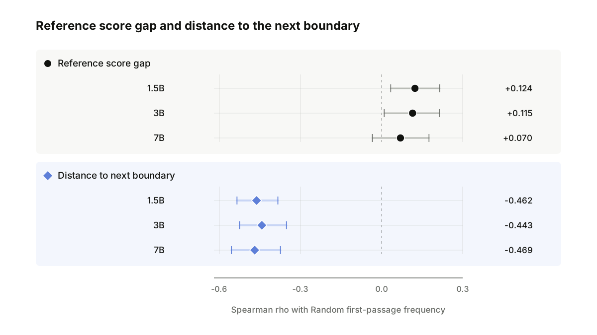
Figure 4. Spearman correlations of Random first-passage frequency with the reference score gap and the pre-training policy's distance to the next boundary. Numbers at right give exact Spearman ρ values; whiskers show pair-cluster bootstrap 95% intervals. Reference score gap had only small correlations of +.070–+.124, whereas next-boundary distance had consistently negative correlations of −.469–−.443.

The two measurements answer different questions. ADM uses a fixed reference measurement to define regions and select training instructions. Distance to the next boundary describes the starting position of each common evaluation pair under the policy being evaluated. These roles should remain distinct when relating the training-data choice to observed learning trajectories.

Timing of Upward Passage

For pairs whose base state was R or U, the analysis compared the first checkpoint at which each pair occupied a state above its base state. The comparison was directly standardized to a common distribution over pre-training state and within-state quartiles of distance to the next boundary. The resulting HighAvg-minus-Random difference in cumulative upward passage was positive from step 92 and was generally largest at step 184 (Table 1).

Model	Step 92	Step 184	Step 276
1.5B	+6.44 pp	+9.28 pp	+8.79 pp
3B	+2.79 pp	+7.64 pp	+5.78 pp
7B	+2.26 pp	+15.11 pp	+13.88 pp

Table 1. HighAvg-minus-Random differences in cumulative upward passage after direct standardization across eight base-state × boundary-distance-quartile strata. Positive values indicate more cumulative upward passage under HighAvg. All nine pair-cluster bootstrap 95% intervals were above zero.

The gap narrowed after step 184, primarily because Random later crossed boundaries that HighAvg had crossed earlier. For 3B, 63 base-U pair-by-seed trajectories had reached T under HighAvg at step 184 while remaining in U under Random. By step 276, 61 of these remained in T under HighAvg, whereas 35 had reached T under Random. The final gap narrowed because of Random’s later catch-up rather than a broad retreat under HighAvg. Figure 5 shows both cumulative passage and the difference across distance-to-next-boundary bins.

Figure 5. The upper panel shows cumulative upward passage standardized across eight base-state × boundary-distance-quartile strata. The lower panel summarizes quartile-specific differences over the 92-step evaluation intervals; larger values indicate a larger cumulative HighAvg advantage over time, not optimizer updates saved. Q1 is closest to the boundary and Q4 farthest; Q4 was weakest for every model.

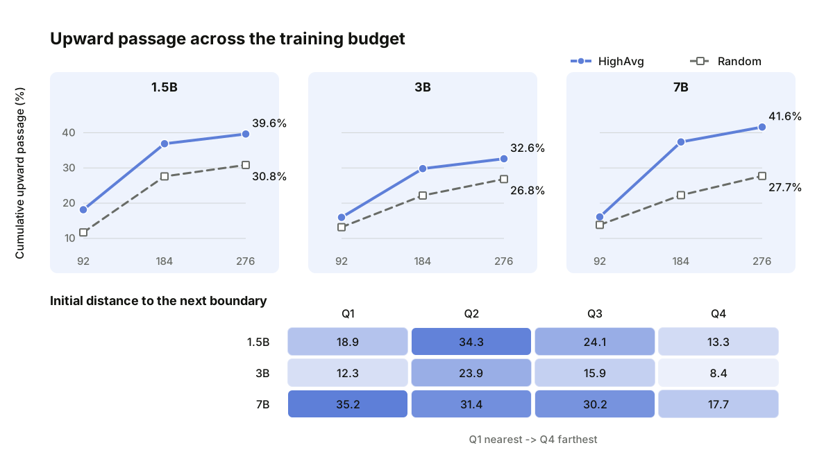
The largest effect did not occur among pairs farthest from the boundary. The HighAvg difference was concentrated in distance ranges from which the pre-training policy could reach the next state within the observation window. The effective distance range was wider for the 7B policy than for the 1.5B and 3B policies, but these three model variants do not establish a monotonic model-size effect.

Here, earlier means that upward passage was observed at an earlier evaluation checkpoint within the same 276-update window. Because checkpoints were evaluated only at steps 92, 184, and 276, the exact optimizer step at which an individual pair crossed a boundary is unknown.

Supporting Evidence from Training Metrics

From epochs 1 to 3, increases in training accuracy and training reward margin were larger under HighAvg than Random for all three models. The change in SimPO loss also favored HighAvg for 1.5B and 7B, while the two conditions were nearly equal for 3B. Exact values and the analysis scope are reported in Appendix Table 1.

The 3B model nevertheless showed differences in the training metrics even though its final upward-movement difference was the smallest. These metrics were measured on different training datasets and do not substitute for trajectories on the shared evaluation set; they serve only as supporting evidence of optimization-related differences between HighAvg and Random at all three model sizes.

Interpretation

The hypothesis that larger models would show a larger HighAvg advantage was not supported monotonically across these three variants. Initial policy state, distance to the next boundary, and the observation budget provide a way to describe the pattern. They form an interpretation of the measured trajectories, rather than an identified causal chain.

Model capacity may still matter. However, the three model variants also differed in their initial R/U/T composition and distances to the next boundary, and those differences more directly described the observed model-specific patterns. This interpretation is consistent with the non-monotonic result—positive HighAvg effects for all three models, larger for 1.5B than 3B, and largest for 7B—and with changes over training. It is also consistent with the effect growing midway through training and then declining as Random caught up later.

A fixed ADM data map identifies the region used to select training data. Policy margins at successive checkpoints describe the trajectories of the common evaluation pairs. Connecting the training-data selection condition to those held-out trajectories yields the central result of this comparison:

HighAvg showed a consistent aggregate advantage in this fixed comparison, but it did not produce a larger improvement for every pair or increase monotonically with model size. Its clearest difference was earlier upward passage across a policy-relative SimPO boundary.

Understanding the learning effect of selected preference data required considering not only the data region, but also the policy’s starting position on each pair and the update window over which its transition was observed.

Limitations

• The shared evaluation set was development data held fixed for the follow-up analysis; whether the same transition pattern persists on a new external evaluation set was not tested.
• The three official model variants differ in training conditions and post-training outcomes as well as parameter count, so the observed differences cannot be interpreted as a pure model-size effect.
• Upward passage was observed only at steps 92, 184, and 276, so the exact optimizer step at which each pair crossed a boundary is unknown.
• Pair-cluster bootstrap intervals condition on the trained runs and resample evaluation pairs. They do not measure uncertainty over a population of training seeds; the resampling unit is the individual pair ID.
• All primary outcomes score supplied response pairs. Generated-answer quality and downstream task performance were not measured in this comparison.

Appendix

Evaluation and Reproduction Conditions

• Source and ADM measurement: The analysis used the same 4,500 UltraFeedback instructions and four candidate responses per instruction as the preceding research note. Reference answers were generated with Qwen3.5-122B-A10B. Candidate responses were measured using overlapping-window mean similarity from all-mpnet-base-v2, and ADM regions were assigned within source × task strata.
• Training data: HighAvg and Random each contained 1,080 instructions, yielding 5,682 and 5,773 valid preference pairs, respectively. The chosen–rejected direction was fixed by fine-grained scores from the source data.
• Training: Training used the SimPO objective with a learning rate of 5e-6, a linear scheduler, and a warmup ratio of 0.1. LoRA used rank 64, alpha 128, and dropout 0.05; cutoff length was 2048, with BF16 precision.
• Exposure: Training ran for 276 optimizer updates with a global batch size of 63, saving checkpoints at steps 92, 184, and 276. Nominal training-pair exposure was 17,388 in both conditions, equivalent to approximately 3 epochs. Step 276 was fixed as the endpoint without checkpoint selection based on results.
• Evaluation: The same 600-pair evaluation set, disjoint from the training data, was used at base and at all three checkpoints. This was fixed development data, not a blind test.
• Analysis: The primary endpoints, upward-passage comparison, and reference–boundary-distance correlation analysis used seeds 42, 43, and 44. The detailed transition decomposition in Figure 3 and the Appendix training-metric table use seed 42. Uncertainty intervals used a pair-cluster bootstrap that resampled pair IDs while preserving repeated observations of the same pair.

Training-Metric Details

HighAvg-minus-Random difference in change from epochs 1→3	1.5B	3B	7B
Training accuracy	+4.06 pp	+2.50 pp	+4.20 pp
Training reward margin $\beta\Delta$	+0.124	+0.130	+0.417
SimPO loss	−0.0343	+0.0039	−0.0333

Appendix Table 1. Seed-42 HighAvg-minus-Random differences in training-metric changes from epochs 1 to 3. Positive differences in training accuracy and reward margin, and negative differences in SimPO loss, favor HighAvg. These are in-distribution supporting metrics measured on different training datasets; they do not substitute for trajectories on the shared evaluation set.

Seed-Level Endpoints on the Shared Evaluation Set

Model	HighAvg accuracy three-seed mean	Random accuracy three-seed mean	Accuracy difference (pp) seeds 42 / 43 / 44	SimPO loss difference seeds 42 / 43 / 44
1.5B	70.06%	68.72%	+1.00 / +1.83 / +1.17	-0.0195 / -0.0228 / -0.0280
3B	72.56%	71.11%	+1.17 / +1.50 / +1.67	-0.0062 / -0.0029 / -0.0051
7B	76.17%	73.17%	+2.50 / +3.83 / +2.67	-0.0336 / -0.0382 / -0.0257

Appendix Table 2. HighAvg-minus-Random differences at step 276 on the same 600 evaluation pairs. Higher accuracy and lower loss are better. These differ from the in-distribution training metrics in Appendix Table 1. The 18 retained evaluation ledgers were SHA-256 checked and their aggregates matched the existing analysis. CSV: per-seed counts, accuracy, and loss.

Final-state movement uses the pooled initial-state distribution across the three models (R 0.350556, U 0.282222, T 0.367222). This is separate from the eight R/U × distance-quartile strata used for Table 1.

Key Metrics

• Policy margin $\Delta$: the policy’s length-normalized chosen–rejected log-probability difference.
• Reward accuracy: the proportion of pairs with $\Delta>0$, meaning that the policy prefers the chosen response to the rejected response.
• Training reward margin: the mean $\beta\Delta$ recorded in the SimPO training logs.
• State-standardized upward movement: the HighAvg-minus-Random difference in the proportion of pairs whose checkpoint state is higher than at base, averaged over base-state-specific differences under a shared R/U/T distribution.
• First observed upward passage: the evaluation checkpoint at which a pair whose base state is R or U first reaches a higher state.
• Distance to the next boundary: the distance from the base margin to the next SimPO boundary: $0-\Delta$ in R and $0.5-\Delta$ in U.
• Base-state × boundary-distance-quartile standardization: a direct weighting procedure that divides eligible pairs into eight strata—two base states and four within-state distance quartiles—and averages condition differences under a common stratum distribution.
• Evaluation-interval summary: a descriptive statistic that summarizes cumulative-passage indicators at steps 92, 184, and 276 as area over 92-step evaluation intervals. It is neither the actual boundary-crossing step nor the number of updates saved.
• Pair-cluster bootstrap: an uncertainty calculation that resamples pair IDs while retaining repeated observations of the same pair within each analysis.

References

1. Lee, S., Kim, E., Lee, H., and Chang, B. Alignment Data Map for Efficient Preference Data Selection and Diagnosis. Findings of ACL 2026, 38225–38241, 2026. ACL Anthology; arXiv
2. Xiao, Y. et al. Finding the Sweet Spot: Preference Data Construction for Scaling Preference Optimization. ACL 2025, 12538–12552, 2025. ACL Anthology
3. Deng, X. et al. Less is More: Improving LLM Alignment via Preference Data Selection. NeurIPS 2025, 161259–161285, 2025. DOI: 10.52202/085713-5383; NeurIPS
4. Yang, S. et al. Not All Preference Pairs Are Created Equal: A Recipe for Annotation-Efficient Iterative Preference Learning. Findings of EMNLP 2024, 6549–6561, 2024. ACL Anthology
5. Huang, K. et al. Larger or Smaller Reward Margins to Select Preferences for LLM Alignment? ICML 2025, 25922–25946, 2025. PMLR
6. Peng, S. et al. Uni-DPO: A Unified Paradigm for Dynamic Preference Optimization of LLMs. ICLR 2026, 2026. OpenReview
7. Li, M., Zhou, X., and Zhao, P. Learning Temporally-Aware Sample Weights for Preference Optimization. Findings of ACL 2026, 12361–12377, 2026. ACL Anthology
8. Li, M., Wang, J., and Zhao, P. What Do LLMs Learn First? Asymmetric Learning Dynamics of Input Complexity and Output Ambiguity in Preference Alignment. ACL 2026, 17373–17388, 2026. ACL Anthology
9. Meng, Y., Xia, M., and Chen, D. SimPO: Simple Preference Optimization with a Reference-Free Reward. NeurIPS 2024, 124198–124235, 2024. NeurIPS

Model and dataset resources: Qwen3.5-122B-A10B, all-mpnet-base-v2, UltraFeedback, Qwen2.5-1.5B-Instruct, Qwen2.5-3B-Instruct, Qwen2.5-7B-Instruct.

Citation

Text citation:

Ilho Ahn, "Alignment Data Map: Timing of SimPO Boundary Crossings and Model-Specific Differences", Mini Research, September 1, 2026.

BibTeX:

@article{ahn2026selectedpreferencepairsearlier,
  author = {Ilho Ahn},
  title = {Alignment Data Map: Timing of SimPO Boundary Crossings and Model-Specific Differences},
  journal = {Mini Research},
  year = {2026},
  month = sep,
  url = {https://muted-color.github.io/research/2026/09/01/selected-preference-pairs-helped-earlier-not-uniformly/}
}